













































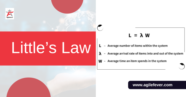
Little’s Law is a fundamental principle in queueing theory and operations research that provides a mathematical relationship between three key metrics: the average number of customers in a system (L), the average arrival rate of customers to the system (λ), and the average time a customer spends in the system (W). This law is named after John D.C. Little, who introduced it in the 1960s.
The formula in team terms
| Symbol | Queueing term | Software team term | Example |
|---|---|---|---|
| L | Average items in the system | Average work in progress (WIP) | 12 items |
| λ | Average arrival rate | Average throughput (items finished per week) | 4 per week |
| W | Average time in the system | Average lead time or flow time | 3 weeks |
12 items = 4 per week × 3 weeks. The example is illustrative.
Little’s Law
Mathematically, Little’s Law can be expressed as:
L = λ * W
Where:
- L represents the average number of customers in the system.
- λ (lambda) represents the average arrival rate of customers to the system (customers per unit of time).
- W represents the average time a customer spends in the system.
Little’s Law essentially states that the average number of customers in a system is equal to the average arrival rate of customers multiplied by the average time each customer spends in the system.
Here’s an intuitive explanation of the components:
- Average Number of Customers (L): This refers to the average number of customers (or items, tasks, etc.) that are present within the system at any given time. In the context of a queue or a process, it’s the average number of entities waiting for service or processing.
- Average Arrival Rate (λ): This represents how many customers, on average, arrive at the system per unit of time. It’s a measure of the input rate or the rate at which work is being requested.
- Average Time in System (W): This is the average amount of time a customer spends within the system, from entering the system to exiting it. It’s the total time spent in queues and undergoing processing.
Little’s Law is a powerful tool used to understand the relationship between these three metrics in various scenarios, such as queuing systems, manufacturing processes, computer networks, and more. It’s especially useful for making predictions and optimizing processes.
For example, if you know the average arrival rate of customers and the average time a customer spends in a system, you can use Little’s Law to estimate the average number of customers in the system. Alternatively, if you know the average number of customers in the system and the average time they spend there, you can use the law to calculate the arrival rate.
In summary, Little’s Law is a simple yet fundamental principle that helps in understanding and analyzing the behaviour of systems involving queues, processes, and customer arrivals, providing insights into the relationship between customer flow, waiting times, and the number of customers in the system.
Interested in the Kanban certification course, check out our website Agilefever.com.
A worked example
A team has 20 items in progress and finishes 5 per week. Average lead time is 20 ÷ 5 = 4 weeks. If the team cuts WIP to 10 items and still finishes 5 per week, average lead time falls to 2 weeks. The team did not work faster. It started less at once, so each item waited less.
When it holds
- The system is stable over the period: work arriving roughly matches work leaving.
- You count every item the same way, with the same start and stop points.
- You use averages over a long enough period, not a single day.
- Items are not abandoned or removed without being counted.
If these do not hold, the numbers will not line up, and that is a useful signal. A WIP count that keeps rising means work is arriving faster than it leaves.
Using it in Kanban
This is the reason Kanban sets WIP limits. With throughput roughly fixed, the fastest way to cut lead time is to lower WIP. Measure all three, and check that the numbers agree. For the measures themselves, see cycle time, lead time and flow time.
Where it applies outside software
| Setting | L | λ | W |
|---|---|---|---|
| Support desk | Open tickets | Tickets closed per day | Average resolution time |
| Change approval | Requests waiting | Approvals per week | Average approval time |
| Code review | Open pull requests | Reviews finished per day | Average time to merge |
Teams that want to apply this with real data can look at the Kanban Systems Improvement (KSI) course (16 hours, $1,100) or the Kanban Management Professional (KMP) certification (32 hours, $2,200).
Additional discounts are available. Contact us to know more.
More questions answered
Who created Little’s Law?
John D. C. Little proved it in 1961, in the context of queueing theory. It is now used in operations, manufacturing and software delivery.
Does Little’s Law work for individual items?
No. It describes averages for a stable system. One item can take much longer or shorter than the average.
Can I use it to forecast?
Only roughly. It tells you how average lead time, throughput and WIP relate. For forecasting a specific delivery date, teams usually use percentiles of past cycle times or simulation.
Last reviewed October 2026 by the AgileFever editorial team.